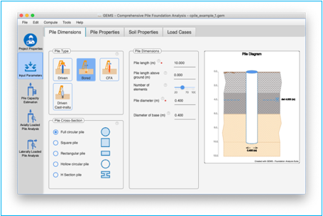
Input Parameters
Input parameters pane specifies the dimensions, properties of the pile, soil, and load cases. These are entered in their respective tabs.
Pile Dimensions Tab
Pile Dimensions tab defines the pile type, cross-section of the pile and the dimensions of the pile for the foundation. It also displays a pictorial view of the pile along with the layers of soil.
Pile Type
Select the pile type (method of construction) used for the project in the pile dimensions tab. The choices for pile types are
a) Driven
b) Bored (Bored cast-insitu)
c) CFA (Continuous flight auger)
d) Driven Cast-insitu
The method of construction along with the pile cross-section and pile material is used to determine the default values for 'k earth pressure coefficient' for sand layers. It is also used in calculation of pile capacity estimation.
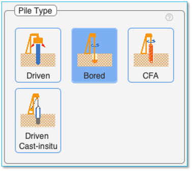
Table 1 below describes the practical choices for pile method of construction, pile cross-section and material used. The application may give warnings (which may be ignored by the user) if the selections don’t adhere to the table below.
Table 1 Pile type, cross-section, material compatibility matrix
|
Pile Type |
Driven |
Bored |
CFA |
Driven Cast-insitu |
|
|
Pile Cross-section |
Hollow Circular H-Section |
Square Rectangular Hollow Circular |
Full Circular |
Full Circular |
Full Circular |
|
Construction material |
Steel |
Concrete |
Concrete |
Concrete |
Concrete |
Pile Cross-Section
Select the pile cross-section to be used for the project in the pile dimensions tab. The choices for pile cross-section are
a) Full circular pile
b) Square pile
c) Rectangular pile
d) Hollow circular pile
e) H Section pile
Based on the cross-section of the pile, define the parameters of the pile in the adjacent pile dimensions pane.
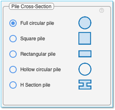
The application may give warnings (which may be ignored by user) if the selections don’t adhere to the Table 1 Pile type, cross-section, material compatibility matrix described in 'Pile Type' section.
Table 2 Summary of parameters to be specified for the different pile cross sections.
|
|
Full Circular pile |
Square pile |
Rectangular pile |
Hollow Circular pile |
H Section pile |
|
Pile length |
✓ |
✓ |
✓ |
✓ |
✓ |
|
Pile length above ground |
Optional |
Optional |
Optional |
Optional |
Optional |
|
Number of elements |
✓ |
✓ |
✓ |
✓ |
✓ |
|
Pile diameter |
✓ |
|
|
✓ |
|
|
Diameter of base |
Optional |
|
|
|
|
|
Pile wall thickness |
|
|
|
✓ |
|
|
Sectional breadth |
|
✓ |
✓ |
|
✓ |
|
Sectional depth |
|
|
✓ |
|
✓ |
|
Sectional area |
|
|
|
|
✓ |
|
Moment of inertia about x-axis |
|
|
|
|
✓ |
|
Moment of inertia about y-axis |
|
|
|
|
✓ |
|
Direction of loading |
|
|
✓ |
|
✓ |
Pile length
Specify the pile length here in the units chosen. After selecting the pile cross-section, this should be the first item to be entered on this page. This field is mandatory for all pile cross-sections.
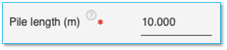
Note: For TRIAL version, Pile length is restricted to 6m (19.6ft)
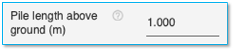
Pile length above ground
Specify the length of the pile length above the ground here in the units chosen. This field is optional and applicable for all pile cross-sections.
Number of elements
This is the guidance of number of elements used in the finite element calculation. The program may adjust this number based on the other input data to carry out the analysis. A higher number of elements will improve granularity but may result in some loss of fidelity. The default value of 50 elements is recommended.
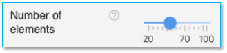
Use the slider to select the number of elements. A minimum of 20 elements and a maximum of 100 elements are permitted. This field is applicable for all pile cross-sections.
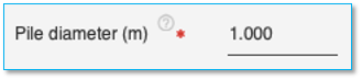
Pile diameter
Specify the external diameter of the pile here in the units specified. This field is mandatory for Full circular pile and Hollow Circular Pile.
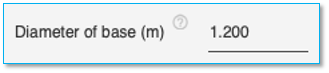
Diameter of base
Specify the diameter of base of the pile here in the units specified if different from the pile diameter. This is usually required for piles with enlarged bases. This field is optional and can be specified only for full circular pile.
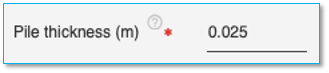
Pile thickness
Specify the pile wall thickness of the pile in the units specified. This field is mandatory and applicable for hollow circular pile.
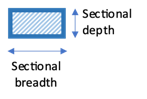
Sectional breadth
Specify the sectional breadth the pile here in the units specified. This field is mandatory for Square pile, Rectangular pile and H Section pile.

Sectional depth
Specify the sectional depth the pile here in the units specified. This field is mandatory for Rectangular pile and H Section Pile.

|
Square Pile |
Rectangular Pile |
H Section Pile |
|
|
|
|


Sectional area
Specify the sectional area the pile here in the units specified. This field is mandatory for H Section pile. The default value displayed here is calculated for a H-section pile with a 1” thickness.

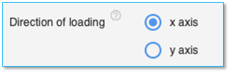
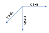
Direction of loading (Required only for lateral pile analysis)
Use the radio button to select the direction of loading of the pile. The choices are x-axis and y-axis. This field is applicable only for Rectangular pile and H-Section piles. The default value is taken as x-axis. The diagram below shows the axis conventions used. The direction of loading will also reflect in the loading diagrams.
|
Rectangular Pile |
H Section Pile |
|
|
|


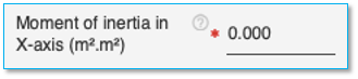
Moment of inertia about X-axis
Specify the moment of inertia of the pile about X-axis here in the units specified. This field is mandatory for H Section Pile.
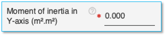
Moment of inertia about Y-axis
Specify the moment of inertia of the pile in Y-axis here in the units specified. This field is mandatory for H Section Pile.
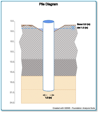
Pile Diagram
The pile diagram displays the pile along with all the layers of soil. Different scales are used for the depth axis and horizontal axis. The pile length in the diagram is 20 m. This diagram shows the perspective view of the pile along with the different layers of soil, scour and depth of water table.
Pile Properties Tab
Pile properties tab is used for specifying the properties of the pile material, pile head boundary conditions, self-weight inputs.

Pile Material Properties
Use the dropdown menu to select the material used for the pile. The elastic modulus of the pile along with the unit weight is updated based on the selection.
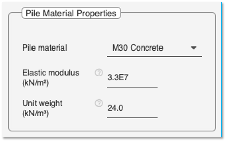
Table 3 Elastic modulus of pile
|
Pile Material |
Elastic Modulus |
|
|
(kN/m3) |
(kips/ft3) |
|
|
Steel |
|
|
|
ASTMA36 |
2.0*108 |
4.173 * 106 |
|
Concrete |
|
|
|
M20 |
3.0 * 107 |
6.26 * 105 |
|
M25 |
3.1 * 107 |
6.47 * 105 |
|
M30 |
3.3 * 107 |
6.68 * 105 |
|
M35 |
3.4 * 107 |
7.10 * 105 |
|
M40 |
3.5 * 107 |
7.31 * 105 |
|
M45 |
3.6 * 107 |
7.52 * 105 |
|
M50 |
3.7 * 107 |
7.73 * 105 |
Select the “User Defined” option to enter values for the elastic modulus and unit weight of the pile material.
Elastic modulus of pile
The elastic modulus of pile is shown here based on the material specified. If “User Defined” material is selected, the elastic modulus of the pile can be edited and entered here.
![]()
Unit weight of material
The unit weight of pile material of pile is shown here based on the material specified. If “User Defined” material is selected, the ‘unit weight of material’ can be edited and entered here.
![]()
Self-weight inputs
The self-weight properties could be considered for axial analysis of the pile.
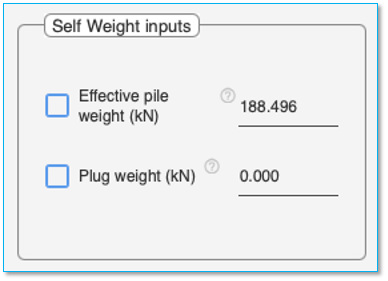
Effective pile weight
The calculated ‘Effective pile weight’ is shown by default. Effective pile weight accounts for the reduction in pile weight due to buoyancy effect of water when a water table is present. To specify a user defined value, select the checkbox and enter the value in the field adjacent to it.

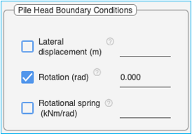
Pile Head Boundary Conditions
The boundary conditions pertain to only lateral analysis of pile and are applied at the pile head.

To specify a boundary condition, select the appropriate checkbox and set the values in the field adjacent to it.
Note: Lateral displacement can be specified only if there are no lateral loads applied at the pile head. This also includes distributed lateral loads starting at the pile head.
Note: Rotation can be specified only if there are no lateral moments applied at the pile head.
Reinforced Section
User calculated axial and flexural rigidity values of reinforced pile section can be specified if required. By default, the calculated values for an un-reinforced pile are displayed.
To specify the axial and flexural rigidity value, select the appropriate checkbox and set the values in the field adjacent to it.

Soil Properties Tab

Soil properties tab is used to enter the details of soil layers, and standard penetration test (SPT) data. The tab is further subdivided into 2 tabs (on right hand side)
· SPT
Soil Properties Tab > Soil Layers Tab
Soil Properties Tab is used to enter the data about the site condition, sub-soil layers and properties of each soil layer. It is divided into 3 panes
This tab is mandatory for ‘Pile Capacity Estimation’, ‘Laterally Loaded Pile Analysis’ and ‘Axially Loaded Pile Analysis’.
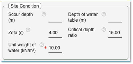
Soil Properties Tab > Soil Layers Tab > Site Condition

Scour depth
This field is not mandatory. Specify the local scour around the pile at the site. Enter the ‘scour’ value in the field.
Some restrictions on the scour depth:
· Scour depth can extend up to the first three layers of soil
· Scour depth should be less than 2.5 times of diameter of the pile
· Scour cannot extend into a rock layer.
Depth of water table
This field is not mandatory. Specify the depth of water table at the site in the field provided.
If no value is specified, it is assumed the water table lies below all the layers of soil specified. For water table at ground level, set it as 0.
Zeta (z)
Specify the value of ‘zeta (z)’ in the field provided.
Zeta (z) is required for Axial load
analysis by ‘Elastic method’ and is based on the parameter proposed by (Randolph and Wroth 1978) as![]() where rm is the radial extent of the influenced zone in
the soil layer due to axil load and ro is the radius of the pile.
where rm is the radial extent of the influenced zone in
the soil layer due to axil load and ro is the radius of the pile.
Min value: 3
Max value: 5
Default value: 4
Critical depth ratio (Zc)
Specify the value of ‘Critical depth ratio’ (zc/d) in the field provided.
Zc is the ratio of depth to diameter of pile beyond which the vertical and lateral effective stresses are considered to remain constant up to the pile base. The usual values are Zc = 15 for loose sand and 20 for dense sand.
Critical depth ratio’ is required for Pile capacity estimation in ‘Sand soil’ when the limiting side friction and base resistance are determined by the values computed at the critical depth. This method is followed in IS-2911 (IS 2911 Design and construction of pile foundations - Code of Practice (Part 1. Sections - 1,2&3) 2010). The software also adopts this method for limiting base resistance determined by ‘Nq - Berezantev – Zc’ method. The table below summarizes the scenarios under which Zc is required.
Analysis Module:
a) Pile capacity analysis
b) Axially loaded pile analysis
Table 4 Scenarios where ‘critical depth ratio’ is required
|
|
Method for maximum base resistance |
|||||
|
Nq - qlim method (API-2011, API-2000) |
Nq-Zc method (IS-2911) |
Nq -Berezantev - Zc method |
Meyerhoff SPT method (IS-2911) |
Meyerhoff SPT method for silty sand (IS-2911) |
||
|
Method for maximum side friction |
β method (API-2011) |
|
✓ |
✓ |
|
|
|
K - δ method (API-2000) |
|
✓ |
✓ |
|
|
|
|
K - δ - Zc method (IS-2911) |
✓ |
✓ |
✓ |
✓ |
✓ |
|
|
Meyerhoff SPT method (IS-2911) |
|
✓ |
✓ |
|
|
|
|
Meyerhoff SPT method for silty sand (IS-2911) |
|
✓ |
✓ |
|
|
|
Min value: 15
Max value: 20
Default value: 15
Unit weight of water
Specify the unit weight of water in the field provided. This parameter is a mandatory field.
Min value: 9.5 kN/m3 or 0.062 kips/ft3
Max value: 10.5 kN/m3 or 0.067 kips/ft3
Default value: 9.8 kN/m3 or 0.063 kips/ft3
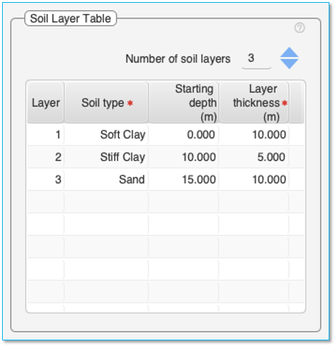
Soil Properties Tab > Soil Layers Tab > Soil Layer Table
The ‘Soil Layer Table’ is used to define the type of soil and the thickness of each layer of soil. The properties of the soil layer selected is entered in the adjacent ‘Soil Layer Properties’ pane.
Number of soil layers
First select the number of soil layers using the up/down arrow. This will set the number of rows in the table to populate
Up 50 soil layers can be specified.
Note: For TRIAL version, number of soil layers is restricted to 3.
Table: Double-click on the table cells to edit the content of the cells.
The table consists of four columns – Layer, Soil type, Starting depth and Layer thickness. The ‘Layer’ column and the ‘Starting depth’ columns cannot be edited.
To enter the Soil type, click on the cell in this column and select the type of soil from the ‘drop down’ menu for each segment.
Permissible soil types currently are – Soft Clay, Stiff Clay, Sand, Weak Rock, and Hard Rock.
You can use ‘Sand’ to represent silt, silty sand, and gravel as well.
Layer thickness Column – This defines the thickness of each layer of soil.
Starting depth Column – This column is auto calculated based on the thickness of soil layers entered.
The pile diagram in the pile dimensions tab will graphically show the values entered in this table.
Note: Soil layers should extend up to pile depth below ground + n * effective diameter
n = 3 for pile terminating in soil
n = 1 for pile terminating in rock.
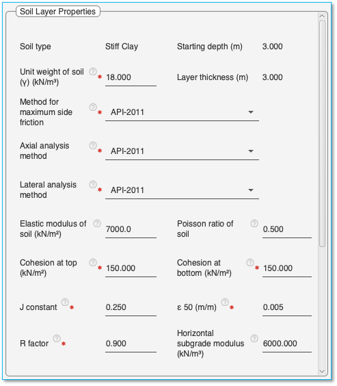
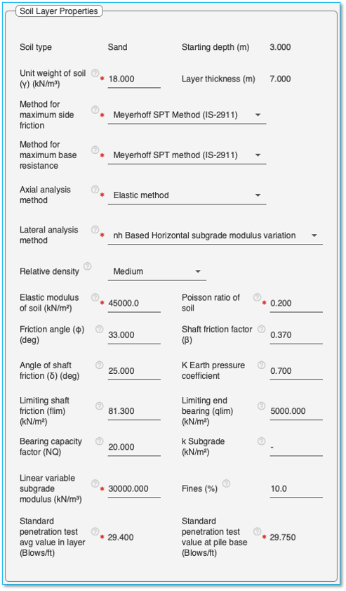
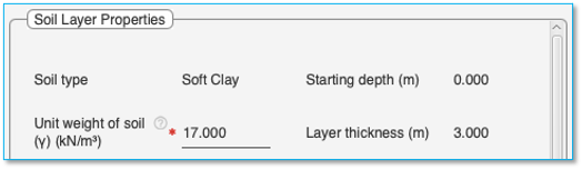
Soil Properties Tab > Soil Layers Tab > Soil Layer Properties
Select a layer in the ‘Soil layer table’ to display the soil properties associated with it in this pane.
Note: Mandatory
fields have a (![]() ) adjacent to them depending on the choices
made for capacity estimation, axial pile analysis and lateral pile analysis.
) adjacent to them depending on the choices
made for capacity estimation, axial pile analysis and lateral pile analysis.
Note: The soil layer properties need to be arrived at from the soil investigation report. The application populates median recommended values for each property. These values need to be updated with actual values from the soil investigation report or values chosen by the user.
Common properties for all soil types:
Soil type: Shows the type of soil in this layer. (Field cannot be edited)
Unit weight of soil (γ): The unit weight to be given as data is the total unit weight of soil in the layer that is the moist unit weight above the water table and saturated unit weight below the water table. If required one may choose to divide the layer in to two halves one above water table and the other below the water table having different unit weights.
Starting depth: Displays the starting depth of the layer. (Field cannot be edited)
Layer thickness: Displays the thickness of the selected layer. (Field cannot be edited)
Properties for Clay soil
Pile capacity estimation of clay soil
Method for maximum side friction: The table below details the options available for Soft Clay and Stiff Clay soil.
Table 5 Details of ‘Method for maximum side friction’ for clay soil
|
Method for maximum side friction |
Notes |
|
API-2011 |
(API 2011 Geotechnical and Foundation Design Considerations April 2011, Addendum 1, 2014) |
|
α method (IS-2911) |
(IS 2911 Design and construction of pile foundations - Code of Practice (Part 1. Sections - 1,2&3) 2010) |
|
Semple & Ridgen (1984) |
(Semple and Rigden 1984) |
|
Kolk & Van Der Velde (1996) |
(Kolk and van der Velde 1996) |
The maximum unit shaft friction tmax of clay soil layers is based on the equation
tmax = α x cu
Where α is a multiplier and cu is the undrained cohesion of the soil. Methods of estimating the α multiplier by the following four methods are available in the software:
1) API RP GEO 2011
In this
α = 0.5 ψ-0.5 ( ψ <= 1.0 )
α = 0.5 ψ-0.25 ( ψ > 1.0 )
ψ = cu / pv' where
cu = undrained shear strength and pv' = vertical effective stress
2) α method (IS 2911)
Curve relating the cu & α given in the Standard is made use of.
3) Semple & Rigden (1984)
tmax (maximum unit shaft friction) = α x F x cu where
α = 1.0 ( ψ <= 0.35 )
α = 1.0 - 0.9 x ( ψ - 0.35) ( 0.35 < ψ < 0.8 )
α = 0.5 ( ψ >= 0.8 )
ψ = cu / pv' where
cu = undrained shear strength and pv' = vertical effective stress
F = 1.0 ( l/d <= 50 )
F = 1.0 – (0.5/70)(l/d – 50) ( 50 < l/d < 120 )
F = 0.7 ( l/d >= 120 )
4) Kolk& van der Velde (1996)
![]()
Base resistance in cohesive soil layers
The unit base resistance is given by
qmax = Nc x cu
Properties for Soft Clay soil
Pile capacity estimation of soft clay soil
Method for maximum side friction: Select the method for maximum side friction from the dropdown list. This parameter is mandatory for Axial pile capacity calculation and Axial loaded pile analysis.
Table 6 Details of ‘Method for maximum side friction’ for soft clay soil
|
Method for maximum side friction |
Notes |
|
API-2011 |
(API 2011 Geotechnical and Foundation Design Considerations April 2011, Addendum 1, 2014) |
|
α method (IS-2911) |
(IS 2911 Design and construction of pile foundations - Code of Practice (Part 1. Sections - 1,2&3) 2010) |
|
Semple & Ridgen (1984) |
(Semple and Rigden 1984) |
|
Kolk & Van Der Velde (1996) |
(Kolk and van der Velde 1996) |
For more details on the methods, refer to the section on 'Method for maximum side friction' under 'Clay Soil'.
Table 7 Required properties for ‘pile capacity estimation’ for soft clay soil.
|
Method for maximum side friction |
Cohesion at top |
Cohesion at bottom |
|
API-2011 |
✓ |
✓ |
|
α method (IS-2911) |
✓ |
✓ |
|
Semple Rigden |
✓ |
✓ |
|
Kolk & Van der Velde |
✓ |
✓ |
Axial analysis method: Select the ‘Axial analysis method’ using the ‘drop down menu’ for axial load analysis.
Table 8 Axial analysis method details for Soft Clay
|
Axial analysis method |
Method details |
|
API-2000 |
(API 2000 RP2A-WSD 2000) |
|
API-2011 |
(API 2011 Geotechnical and Foundation Design Considerations April 2011, Addendum 1, 2014) |
|
Elastic method |
Based on elastic properties of soil. |
Table 9 Required properties for ‘axial pile analysis’ for soft clay soil.
|
Axial analysis method |
Cohesion at top |
Cohesion at bottom |
R factor |
Elastic modulus |
Poisson ratio |
|
API-2011 |
✓ |
✓ |
✓ |
||
|
API-2000 |
✓ |
✓ |
✓ |
||
|
Elastic Code |
✓ |
✓ |
✓ |
✓ |
Lateral analysis method: Select the ‘Lateral analysis method’ using the ‘drop down menu’ for lateral load analysis.
Table 10 Lateral analysis method details for Soft Clay
|
Lateral analysis method |
Method details |
|
API-2011 |
(API 2000 RP2A-WSD 2000) |
|
kh Based Horizontal Subgrade Modulus |
Lateral spring of constant stiffness based on kh
IS-2911 recommends use of kh based horizontal subgrade modulus method for lateral analysis of pile. (IS 2911 Design and construction of pile foundations - Code of Practice (Part 1. Sections - 1,2&3) 2010) |
|
nh Based Horizontal Subgrade Modulus Variation |
Lateral spring of stiffness proportional to depth based on nh
IS-2911 recommends use of nh based horizontal subgrade modulus variation method for lateral analysis of pile. (IS 2911 Design and construction of pile foundations - Code of Practice (Part 1. Sections - 1,2&3) 2010) |
1. API 2011 recommends nonlinear p-y models for static and cyclic loading. The parameters used in the model are undrained cohesion cu, ε50 strain at 50% maximum lateral stress pu and a factor J.
2. kh based method on Horizontal Subgrade Modulus: IS 2911 has provided recommended values for use in this method
3. Linear elastic spring model based on nh: In this approach the lateral soil resistance is proportional to depth given by p/y = nh x z where z is the depth.
Recommended values of nh (Davisson 1970) are :
Soft normally-consolidated clays: 350 to700 kN/m3
Soft organic silts: 150kN/ m3. The input required for this method is the value of nh for the soil layer.
IS-2911 has provided recommended values for use in this method
Table 11 Required properties for lateral pile analysis for soft clay soil.
|
Lateral analysis method |
Cohesion at top |
Cohesion at bottom |
J constant |
ε 50 |
Horizontal subgrade modulus |
Linear variable subgrade modulus |
|
API-2011 |
✓ |
✓ |
✓ |
✓ |
|
|
|
kh Based Horizontal Subgrade Modulus |
|
|
|
|
✓ |
|
|
nh Based Horizontal Subgrade Modulus Variation |
|
|
|
|
|
✓ |
Table 12 Soil property details for soft clay soil
|
Soil property |
Units |
Min value |
Max value |
Notes |
|
Elastic modulus of soil |
kN/m2 |
1750 |
5000 |
|
|
kips/ft2 |
36.54 |
104.4 |
||
|
Poisson Ratio |
|
0.1 |
0.5 |
Default value: 0.5 |
|
Cohesion at top |
kN/m2 |
0 |
100 |
Value of 0 is only permissible for the first soil layer. |
|
kips/ft2 |
0 |
2.09 |
||
|
Cohesion at bottom |
kN/m2 |
> 0 |
100 |
|
|
kips/ft2 |
> 0 |
2.09 |
||
|
J Constant |
|
0.25 |
0.5 |
Default value: 0.5 |
|
e 50 |
|
> 0 |
0.025 |
Default value: 0.01 |
|
R factor |
|
0.5 |
1.0 |
Default value: 0.9 |
|
Horizontal subgrade modulus |
kN/m3 |
> 500 |
|
|
|
kips/ft3 |
> 10 |
|
||
|
Horizontal subgrade modulus variation |
kN/m3 |
> 10 |
1000 |
|
|
kips/ft3 |
> 0.25 |
21 |
Properties for Stiff Clay soil

Pile capacity estimation of stiff clay
Method for maximum side friction: Select the method for maximum side friction from the dropdown list. This parameter is mandatory for Axial pile capacity calculation and Axial loaded pile analysis.
Table 13 Details of ‘Method for maximum side friction’ for stiff clay soil
|
Method for maximum side friction |
Notes |
|
API-2011 |
(API 2011 Geotechnical and Foundation Design Considerations April 2011, Addendum 1, 2014) |
|
α method (IS-2911) |
(IS 2911 Design and construction of pile foundations - Code of Practice (Part 1. Sections - 1,2&3) 2010) |
|
Semple & Ridgen (1984) |
(Semple and Rigden 1984) |
|
Kolk & Van Der Velde (1996) |
(Kolk and van der Velde 1996) |
For more details, refer to the section on 'Method for maximum side friction' under 'Clay Soil'.
Table 14 Required properties for ‘pile capacity estimation’ for stiff clay soil.
|
Method for maximum side friction |
Cohesion at top |
Cohesion at bottom |
|
API-2011 |
✓ |
✓ |
|
α method (IS-2911) |
✓ |
✓ |
|
Semple Rigden |
✓ |
✓ |
|
Kolk & Van der Velde |
✓ |
✓ |
Axial analysis method: Select the ‘Axial analysis method’ using the ‘drop down menu’ for axial load analysis.
Table 15 Axial analysis method details for stiff clay
|
Axial analysis method |
Method details |
|
API-2000 |
(API 2000 RP2A-WSD 2000) |
|
API-2011 |
(API 2011 Geotechnical and Foundation Design Considerations April 2011, Addendum 1, 2014) |
|
Elastic method |
Based on elastic properties of soil. |
Table 16 Required properties for ‘axial pile analysis’ for stiff clay soil.
|
Axial analysis method |
Cohesion at top |
Cohesion at bottom |
R factor |
Elastic modulus |
Poisson ratio |
|
API-2011 |
✓ |
✓ |
✓ |
||
|
API-2000 |
✓ |
✓ |
✓ |
||
|
Elastic Code |
✓ |
✓ |
✓ |
✓ |
Lateral analysis method: Select the ‘Lateral analysis method’ using the ‘drop down menu’ for lateral load analysis.
Table 17 Lateral analysis method details for stiff clay
|
Lateral analysis method |
Method details |
|
API-2011 |
(API 2011 Geotechnical and Foundation Design Considerations April 2011, Addendum 1, 2014) |
|
REESE |
(Reese and Cox, Field Testing and Analysis of Laterally Loaded Piles in Stiff Clay April 1975) |
|
kh Based Horizontal Subgrade Modulus |
Lateral spring of constant stiffness based on kh
IS-2911 recommends use of kh based horizontal subgrade modulus method for lateral analysis of pile. (IS 2911 Design and construction of pile foundations - Code of Practice (Part 1. Sections - 1,2&3) 2010) |
1. API-2011 recommends nonlinear p-y models for static and cyclic loading. The parameters used in the model are undrained cohesion cu, ε50 strain at 50% maximum lateral stress pu and a factor J.
2. Reese model
This is also a non-linear p-y model for static and cyclic loading (Reese,Cox,Koop-1975). The soil parameters needed are cu, ε 50 strain at 50% maximum lateral stress pu .The model is applicable to only layers below water table.
3. Method based on horizontal subgrade modulus kh of the soil layer.
This is a linear spring model and the kh should include the correction ( division by 1.5) for use in piles. In SI units the value should be for 1m x 1m and in American units for 1ft x 1ft of pile The values kh recommended by Terzaghi (1955) for pile width are given Table 18 & Table 19 below.
Table 18 kh values for 1ft width & 1ft length of pile (Terzaghi, 1955)
|
Consistency |
Stiff |
Very stiff |
Hard |
|
qu(tsf) |
1 -2 |
2-4 |
>4 |
|
Kh(tcf) |
50 |
100 |
>200 |
The values in SI units after width correction for 1m are given below:
Table 19 Modified Terzaghi values of kh for 1 m width & 1m length of pile in SI units
|
Consistency |
Stiff |
Very stiff |
Hard |
|
qu (kPa) |
100-200 |
200-400 |
>400 |
|
kh(kN/m3) |
5300 |
10500 |
>21000 |
IS-2911 also has given recommendations for kh values.
Modified Vesic’s equation for piles (Bowels 1968)
![]()
Table 20 Required properties for laterally loaded pile analysis for stiff clay soil
|
Lateral analysis method |
Cohesion at top |
Cohesion at bottom |
J constant |
ε 50 |
Horizontal subgrade modulus |
|
API-2011 |
✓ |
✓ |
✓ |
✓ |
|
|
REESE |
✓ |
✓ |
|
✓ |
|
|
kh based Horizontal Subgrade Modulus |
|
|
|
|
✓ |
Table 21 Soil property details for stiff clay soil
|
Soil property |
Units |
Min value |
Max value |
Notes |
|
Elastic modulus of soil |
kN/m2 |
4000 |
10000 |
|
|
kips/ft2 |
83.5 |
208.8 |
||
|
Poisson Ratio |
|
0.1 |
0.5 |
Recommended value Below water table: 0.5 Above water table: 0.4 |
|
Cohesion at top |
kN/m2 |
100 |
|
For the top layer, a value from 0 can be used. |
|
kips/ft2 |
2.09 |
|
||
|
Cohesion at bottom |
kN/m2 |
100 |
|
|
|
kips/ft2 |
2.09 |
|
||
|
J Constant |
|
0.25 |
0.5 |
Default value: 0.25 |
|
ε 50 |
|
> 0 |
0.025 |
Default value: 0.005 |
|
R factor |
|
0.5 |
1.0 |
Default value: 0.9 |
|
Horizontal subgrade modulus |
kN/m3 |
> 1000 |
|
|
|
kips/ft3 |
> 21 |
|
Properties for Sand soil

Pile capacity estimation of sand
Method for maximum side friction: Select the method for maximum side friction from the dropdown list. This parameter is mandatory for Pile capacity estimation calculation and Axial loaded pile analysis. The table below details the options available for Sand soil.
Table 22 Details of ‘Method for maximum side friction’ for sand
|
Method for maximum side friction |
Notes |
|
β method (API-2011) |
(API 2011 Geotechnical and Foundation Design Considerations April 2011, Addendum 1, 2014) |
|
K - δ method (API-2000) |
(API 2000 RP2A-WSD 2000) |
|
K - δ - Zc method (IS-2911) |
(IS 2911 Design and construction of pile foundations - Code of Practice (Part 1. Sections - 1,2&3) 2010) |
|
Meyerhoff SPT method (IS-2911) |
(IS 2911 Design and construction of pile foundations - Code of Practice (Part 1. Sections - 1,2&3) 2010) |
|
Meyerhoff SPT method for silty sand (IS-2911) |
(IS 2911 Design and construction of pile foundations - Code of Practice (Part 1. Sections - 1,2&3) 2010) |
1) The β - fmax method (API-2011)
In this method tmax is given by the equation tmax = b x pv' in which β depends on the density of the sand layer and pv' is the vertical effective stress. β values recommended by API range from 0.29 for medium dense sand to 0.56 for very dense sand. User defined value β could also be specified. This method requires also a value of flim which is the limiting value for tmax. API proposes flim values ranging from 67 kPa for medium dense sand to 115 kPa for very dense sand. User defined value of flim could also be prescribed.
2) K - δ - flim method (API-2000)
In this method tmax is given by the equation tmax = K x tanδ x pv' in which K is lateral earth pressure coefficient, d is the angle of friction between the pile surface and soil and pv' is the vertical effective stress. The values of K and δ need to be specified by the user after due consideration of type of soil, pile and method of installation. Some guidance values in this regard are given in the appendix. API recommends a K value of 0.8 for open ended pipe piles and 1.0 for closed ended piles. The recommended δ values range from 15 degrees for very loose sand to 35 degrees for very dense sand. Standards and literature would be of help in choosing the appropriate values of K and δ. K and δ displayed in the software are those recommended by the code for driven tubular piles.
3) K - δ - Zc method (IS 2911)
In this method tmax is given by the equation tmax = K x tan δ x pv'.The maximum vertical effective stress pv' is limited to the value at the critical depth Zc. Zc /D ratio is specified ranging from 15 for φ' <= 30° to 20 for φ' >=40°. There is provision for user defined values of δ, K and Zc
4) Meyerhoff SPT method (IS 2911)
In this method ![]() for sand and
for sand and ![]() for silty sand where
for silty sand where ![]() is the average N value for the layer.
is the average N value for the layer.