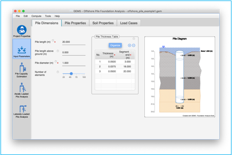
Input Parameters

Input parameters pane specifies the dimensions, properties of the pile, soil, and load cases.  These are entered in their respective tabs. 

Pile Dimensions Tab

Pile Dimensions tab defines the dimensions of the pile for the foundation.  It also displays a pictorial view of the pile along with the layers of soil.    

Pile Length

Specify the length of the pile here in the units chosen.  This should be the first item to be entered on this page.  This field is mandatory.

Note: For TRIAL version, Pile length is restricted to 20m (65.6ft)

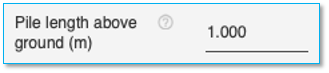
Pile length above ground

Specify the length of the pile length above the ground here in the units chosen.  This field is optional.

Pile diameter

Specify the external diameter of the pile here in the units specified.  The cross-section is assumed to be annular circular pile having uniform external diameter.  This field is mandatory.

Number of elements

This is the guidance of number of elements used in the finite element calculation.  The program may adjust this number based on the other input data to carry out the analysis.  A higher number of elements will improve granularity but may result in some loss of fidelity.  The default value of 50 elements is recommended. 

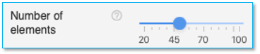
Use the slider to select the number of elements. A minimum of 20 elements and a maximum of 100 elements are permitted.

Pile Thickness Table

The pile thickness table is used to define the pile wall thickness of each segment of the pile.  This table is mandatory.

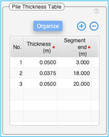
Use the (+) and (-) buttons at the top of the table to add / delete rows to the Pile thickness table. 

[Organize] button can be used to sort the values in ascending order of 'Segment end' and to clean up empty entries in the table. 

Up 20 thickness segments can be defined.

Table:

You can double-click on the table cells to edit the content of the cells.

The table consists of two editable columns –Thickness and Segment end. 

Thickness Column - Click on the cell in this column and enter the value of thickness for the segment.  

Segment end Column – This defines the end value of each segment. For the first segment the beginning value is automatically assigned as zero. For all other segment the beginning values is automatically assigned the value corresponding to the end of the previous segment. For the last segment it is mandatory to assign a value equal to the pile length.

The pile diagram in the pile dimensions tab graphically shows the values entered in this table. 

Pile Diagram

The pile diagram displays the pile along with all the layers of soil.  Different scales are used for the depth axis and horizontal axis.

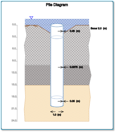
Values of pile wall thickness are shown in the corresponding pile segment.  Pile length in the diagram is 20 m as specified before. 

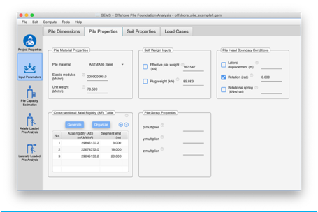
Pile Properties Tab

Pile properties tab is used for specifying the properties of the pile material, self-weight parameters, pile head boundary conditions, cross-sectional axial rigidity and pile group properties. 

Pile material properties

Use the dropdown menu to select the material used for the pile.  The elastic modulus of the pile along with the unit weight is updated based on the selection.

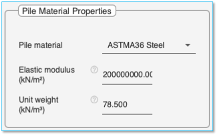
Table of Elastic modulus of pile

Pile Material	Elastic Modulus
	(kN/m^3)	(kips/ft^3)
Steel
ASTMA36	2.0*10^8	4.173 * 10^6
Concrete
M20	3.0 * 10^7	6.26 * 10^5
M25	3.1 * 10^7	6.47 * 10^5
M30	3.3 * 10^7	6.68 * 10^5
M35	3.4 * 10^7	7.10 * 10^5
M40	3.5 * 10^7	7.31 * 10^5
M45	3.6 * 10^7	7.52 * 10^5
M50	3.7 * 10^7	7.73 * 10^5

Select the “User Defined” option to enter values for the elastic modulus and unit weight of the pile material. 

Elastic modulus of pile

The elastic modulus of pile is shown here based on the material specified.  If “User Defined” material is selected, the elastic modulus of the pile can be edited and entered here. 

Unit weight of material

The unit weight of pile material of pile is shown here based on the material specified.  If “User Defined” material is selected, the ‘unit weight of material’ can be edited and entered here.

Self-weight inputs

The self-weight properties could be taken into account for axial analysis of the pile.  The values of self-weight are auto-calculated based on the pile dimensions and soil properties or they could be user-defined. 

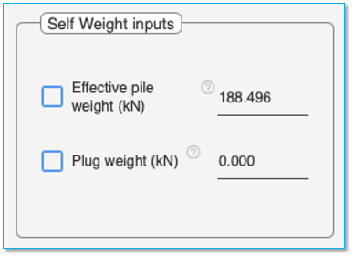
Effective pile weight

The automatically calculated ‘Effective pile weight’ is shown here as default value. Effective pile weight accounts for the reduction in pile weight due to buoyancy effect of water. This will be used for ‘self-weight’ analysis if required. To enter a user defined value of ‘effective pile weight’, select the checkbox adjacent to this and enter the user defined value in the ‘text field’ next to it.  

Plug weight

The automatically calculated plug weight is shown here by default.  The automatic calculation is based on the different soil layers and the inner diameter of the bottom segment of the pile.  A 0.9 reduction factor is used in calculating the plug weight.  This will be used for ‘self-weight’ analysis if required.  To enter a user defined value of plug-weight, select the checkbox adjacent to this and enter the user defined values in the ‘text field’ next to it.  

Pile Head Boundary Conditions

The boundary conditions are applicable for lateral analysis of pile and are applied at the pile head. 

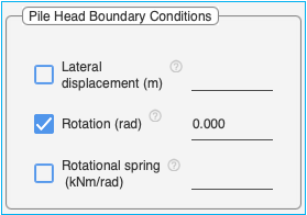
Lateral Displacement

Select the checkbox ‘Lateral displacement’ to set the lateral ‘pile head’ displacement.  Enter the lateral displacement value in the field provided. 

Note: Lateral displacement can be specified only if there are no lateral loads applied at the pile head. This also includes distributed lateral loads starting at the pile head. 

Rotation

Select the checkbox ‘Rotation’ to set the ‘pile head’ rotation.  Enter the rotation value (radians) in the field provided. 

Note: Rotation can be specified only if there are no lateral moments applied at the pile head.

Rotational spring

Select the checkbox ‘Rotational spring’ to set the ‘pile head’ rotational spring value.  Enter the rotational spring value in the field provided. 

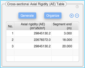
Cross-sectional Axial Rigidity (AE) Table

The cross-sectional axial rigidity (AE) table can be used for specifying user-defined values of AE for different segments of the pile. If the table is left blank the software will auto-calculate the AE values based on the young’s modulus E and wall thickness of each segment of the pile.  This table provides a facility to consider composite sections of pile. It is necessary to provide AE values till the pile tip if specified.

Populating this table is OPTIONAL.

AE of a hollow cylindrical section of a pile is calculated as

AE =  E

D – Diameter of the pile

th – Thickness of the pile segment

E – Elastic modulus the pile material

AE for composite sections is calculated as

AE = AE1 + AE2

Use the (+) and (-) buttons at the top of the table to add / delete rows to the axial rigidity table. 

[Generate] button is provided for convenience.  Click to generate the AE values for the pile based on the pile dimensions and elastic constant of the pile.  The AE values will only be generated if the existing AE table is empty, and the pile dimension parameters and elastic constant of the pile are valid.  The AE value of each segment is calculated using the AE formula described above.

[Organize] button can be used to sort the values in ascending order of 'Segment end' and to clean up empty entries in the table. 

Up 20 cross-sectional axial rigidity segments can be defined.

Table:

You can double-click on the table cells to edit the content of the cells.

The table consists of two editable columns – Axial rigidity (AE) and Segment end. 

Axial rigidity (AE) - Double click on the cell in this column and enter the value of the cross-sectional axial rigidity for the segment. 

Segment end Column - This defines the end value of each segment. For the first segment the beginning value is automatically assigned as zero. For all other segment the beginning values is automatically assigned the value corresponding to the end of the previous segment. For the last segment it is mandatory to assign a value equal to the pile length.

Pile Group Properties

Group effect could be included in the axial pile analysis by specifying the user defined parameter z-multiplier. Similarly group effect in lateral pile analysis could be considered by specifying user defined y-multiplier. Shadowing effect in lateral pile analysis could be considered user specified p-multiplier.                                       

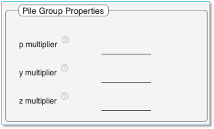
p Multiplier

Enter the value for ‘p multiplier’ the field provided.  The ‘p’ value in the ‘p-y tables’ is multiplied by this value prior to the analysis.  This is an optional parameter.

y Multiplier

Enter the value for ‘y multiplier’ the field provided.  The ‘y’ value in the ‘p-y tables’ is multiplied by this value prior to the analysis.  This is an optional parameter.

z Multiplier

Enter the value for ‘z multiplier’ the field provided.  The ‘z’ value in the ‘t-z tables’ is multiplied by this value prior to the analysis.  This is an optional parameter.

Soil Properties Tab

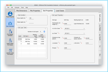
Soil properties tab is used to enter the details of soil layers, enter / compute p-y, t-z and Q-z data.  The tab is further subdivided into 5 tabs (on right hand side)

· Soil Layers

· p-y-Static

· p-y-Cyclic

· t-z

· Q-z

Soil Properties Tab > Soil Layers Tab

Soil Layers tab is used to enter the data about the site condition, sub-soil layers and properties of each soil layer.  It is divided into 3 panes

· Site Condition

· Soil Layer Table

· Soil Layer Properties

This tab is mandatory for ‘Pile Capacity Estimation’.  This tab is mandatory if ‘p-y’ tables need to be auto-generated for ‘Lateral Analysis of Pile’.  This tab is also mandatory if ‘t-z’ or ‘Q-z’ tables need to be auto-generated for ‘Axial Pile Analysis’.      

Soil Properties Tab > Soil Layers Tab > Site Condition

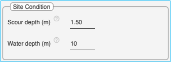
Scour depth

This field is not mandatory. Specify the local scour around the pile at the site.  Enter the ‘scour’ value in the field. 

Some restrictions on the scour depth:

· Scour depth can extend up to the first three layers of soil

· Scour depth should be less than 2.5 times of diameter of the pile

· Scour cannot extend into a rock layer.

Water depth

This field is not mandatory. Specify the water depth at the site. This will be used to adjust the effective weight of the pile. 

Soil Properties Tab > Soil Layers Tab > Soil layer table

The soil layer table is used to define the type of soil and the thickness of each layer of soil. The properties of the soil layer selected is entered in the adjacent ‘Soil Layer Properties’ pane. 

This table is mandatory under the following conditions:

1. Pile Capacity Estimation needs to be performed.

2. If ‘p-y’ tables need to be auto-generated for ‘Lateral Analysis of Pile’. 

3. If ‘t-z’ or ‘Q-z’ tables need to be auto-generated for ‘Axial Analysis of Pile’.

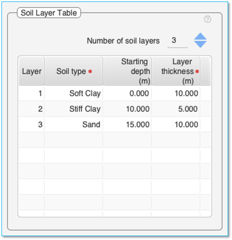
Number of soil layers

First select the number of soil layers using the up/down arrow.  This will set the number of rows in the table to populate

Up 50 soil layers can be specified.

Note: For TRIAL version, number of soil layers is restricted to 3.

Table:

You can double-click on the table cells to edit the content of the cells.

The table consists of two editable columns Soil type and Layer thickness. 

To enter the Soil type, click on the cell in this column and select the type of soil from the ‘drop down’ menu for each segment.

Permissible soil types currently are – Soft Clay, Stiff Clay, Sand, Weak Rock and Hard Rock.    

You can use ‘Sand’ to represent silt and gravel as well.

Layer thickness Column – This defines the thickness of each layer of soil.

Starting depth Column – This column is auto calculated based on the thickness of soil layers entered. 

The pile diagram in the pile dimensions tab shows the values entered in this table. 

Note: Soil layers should extend up to pile depth below ground + n * diameter

n = 3 for pile terminating in soil

n = 1 for pile terminating in rock.

Soil Properties Tab > Soil Layers Tab > Soil layer properties

Select a layer in the ‘Soil layer table’ to display the soil properties associated with it in this pane. 

Note: Mandatory fields have a () adjacent to them

Note: The soil layer properties need to be arrived at from the soil investigation report.  The application populates median recommended values for each property.  These values need to be updated with actual values from the soil investigation report or values chosen by the user.

Common properties for all soil types:

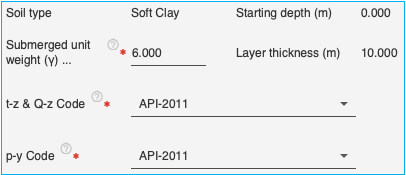
Soil type: Shows the type of soil in this layer.  (Field cannot be edited)

Submerged unit weight (γ): submerged unit of soil in the layer.

Starting depth: Displays the starting depth of the layer. (Field cannot be edited)

Layer thickness: Displays the thickness of the selected layer.  (Field cannot be edited)

t-z & Q-z Code: Select the t-z & Q-z code using the ‘drop down menu’ for pile capacity calculation and axial load analysis.  The table below details the selectable t-z & Q-z practices for the various soil types. Only the relevant recommended practice is displayed based on the soil type selected in the layer. 

Soil Type	t-z & Q-z Code	t-z & Q-z Code details
Soft Clay	API-2000	API RP2A –WSD 21^st Edition Dec.2000
	API-2011	Geotechnical and Foundation Design Considerations ANSI/API RP 2GEO, 1^st Ed, April 2011 Addendum 1,  Oct.2014
Stiff Clay	API-2000	API RP2A –WSD 21^st Edition Dec.2000
	API-2011	Geotechnical and Foundation Design Considerations ANSI/API RP 2GEO, 1^st Ed, April 2011 Addendum 1,  Oct.2014
Sand	API-2000	API RP2A –WSD 21^st Edition Dec.2000
	API-2011	Geotechnical and Foundation Design Considerations ANSI/API RP 2GEO, 1^st Ed, April 2011 Addendum 1,  Oct.2014
Weak Rock	Other	Adaptation based on Piling Engineering by Fleming et al, 3^rd Ed, 2009, Taylor & Francis.
Hard Rock	Other	Adaptation based on Piling Engineering by Fleming et al, 3^rd Ed, 2009, Taylor & Francis.

p-y Code: Select the p-y code using the ‘drop down menu’ for lateral load analysis and p-y curve generation.  The table below details the p-y codes for the various soil types. Only the relevant recommended practices is displayed based on the soil type selected in the layer.

Soil Type	p-y Code	p-y Code details
Soft Clay	API-2011	API RP2A –WSD 21^st Edition Dec.2000
Stiff Clay	API-2011	Geotechnical and Foundation Design Considerations ANSI/API RP 2GEO, 1^st Ed, April 2011 Addendum 1,  Oct.2014
	REESE	REESE, L. C. and COX, W. R. (1975), Field Testing and Analysis of Laterally Loaded Piles in Stiff Clay. Proc. 5th Annual Offshore Technology Conf., OTC 2312, Houston, Texas, April, 1975.
Sand	API-2011	Geotechnical and Foundation Design Considerations ANSI/API RP 2GEO, 1^st Ed, April 2011 Addendum 1,  Oct.2014
	Hybrid model for liquefied sand (Based on φ)	Hybrid model for liquified sand can be used for modelling laterally loaded pile behaviour in sand layers due to liquefaction after an earthquake. This model is based on the paper: Franke, Kevin W, and Rollins M Kyle. “Simplified hybrid p-y spring model for liquified soils.” Geotechnical and Geo-environmental Eng., no. 139(4) (2013): 564-576. This model makes use of the friction angle (φ) of layer Note: This model is available only with SI unit system
Weak Rock	REESE	REESE, L. C. 1997. Analysis of Laterally Loaded Piles in Weak Rock. Journal of Geotechnical and Geo-environmental Engineering, 123, 1010-1017.
Hard Rock	TURNER (2006)	Turner, J. Rock-Socketed Shafts for Highway Structure Foundations. In:Program, N.C.H.R (Ed) A Synthesis of Highway Practice, Transportation Research Board of the National Academies, 2006.

Properties for Clay soil

Properties for Soft Clay soil

Property	Units	Min Value	Max Value	Notes
Cohesion at top	kN/m^2	0	100	Value of 0 is only permissible for the first soil layer.
	kips/ft^2	0	2.09
Cohesion at bottom	kN/m^2	>0	100
	kips/ft^2	>0	2.09
J Constant		0.25	0.5	Default value: 0.5
ε 50		> 0	0.025	Default value: 0.01
R factor		0.5	1.0	Default value: 0.9

Properties for Stiff Clay soil

Property	Units	Min Value	Max Value	Notes
Cohesion at top	kN/m^2	100
	kips/ft^2	2.09
Cohesion at bottom	kN/m^2	100
	kips/ft^2	2.09
J Constant		0.25	0.5	Default value: 0.25
ε 50		> 0	0.025	Default value: 0.005
R factor		0.5	1.0	Default value: 0.9

Properties for Sand soil

Relative density:  Select the relative density of the sand soil from the dropdown menu.  The choices are ‘Very Loose’, ‘Loose’, ‘Medium’, ‘Dense’ and ‘Very Dense’ sand.  Based on the relative density selection and the ‘t-z Code’ selected, the application populates the recommended values for the below parameters based on the appropriate API recommended practices.  These values can be replaced by user preferred values.

Note: For ‘Very Loose’ and ‘Loose’ sand, t-z/Q-z API-2011 code doesn’t recommend any values for ‘Shaft friction factor’, ‘Limiting shaft friction (flim), Limiting end bearing (qlim) and Bearing capacity factor (NQ).  These need to be prescribed by the user based on soil investigation reports.

Property	Units	Min Value	Max Value	Notes
Friction angle (φ)	Deg	5	60	The value is not changed based on selection of ‘relative density of soil’
Shaft friction factor (β)		0.10	1.0	For API-2011 code only
Angle of shaft friction (δ)	Deg	5	45	For API-2000 code only
K Earth pressure coefficient		0.5	1.2	For API-2000 code only
Limiting shaft friction (flim)	kN/m^2	0	120
	kips/ft^2	0	2.5
Limiting end bearing (qlim)	kN/m^2	0	15000
	kips/ft^2	0	313.2
Bearing capacity factor (NQ)		1.5	320
Fines	%	0	75	Percentage of fine particle sand
K subgrade		>0		K-subgrade may be specified if available.  Otherwise, the program calculates the values based on the friction angle provided.  Set the value as – to enable auto calculation.

Properties for Weak Rock

Property	Units	Min Value	Max Value	Notes
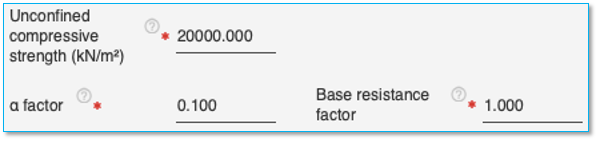
Unconfined compressive strength	kN/m^2	1000	20000
	kips/ft^2	20.88	417.6
α factor	(kN/m^2)^1/2	3	20	Focht Jr., John A. Koch, Kenneth. J. “Rational Analysis of the Lateral Performance of Offshore Pile Groups.” Offshore Technology Conference. 1973. Paper N0 1896.
	(kips/ft^2)^1/2	0.433	2.89
Base resistance factor		0.5	3	Reese, et al. “Analysis of a Pile Group under Lateral Loading, Laterally Loaded Deep Foundations: Analysis and Performance.” ASTM, STP 835, 1984: 56-71.
Rock quality designation	%	0	100
KRML constant		0.00005	0.0005
Elastic modulus of rock	kN/m^2	1000000	20000000	Typically1000 * Unconfined compressive strength of rock
	kips/ft^2	20885	417708

Properties for Hard rock

Property	Units	Min Value	Max Value	Notes
Unconfined compressive strength	kN/m^2	10000	100000
	kips/ft^2	208.8	2088
α factor		3	20
Base resistance factor		0.2	3

Soil Properties Tab > p-y-Static Tab & p-y-Cyclic Tab

Note: p-y curves are required if ‘Laterally Loaded Pile Analysis’ is selected in the Project Properties Tab.  Data in this tab is not used otherwise and can be skipped altogether if only ‘Pile Capacity’ or ‘Axially Loaded Pile Analysis’ is required. 

p-y-Static tab contains the data for the p-y curves under static loading for the project.  This is required if any of the ‘Load Cases’ in the ‘Load Cases Tab’ contains ‘Static’ loading.

p-y-Cyclic tab contains the data for the p-y curves under cyclic loading for the project.  This is required if any of the ‘Load Cases’ in the ‘Load Cases Tab’ contains ‘Cyclic’ loading.

The below section holds good for p-y curves for Static & Cyclic loading.  The two tabs are independent of one another.

The p-y curves can either be (a) auto-generated from ‘soil properties’ and ‘pile dimensions’ data or (b) user-defined. 

Auto-generate p-y Curves: Select this checkbox to autogenerate the p-y curves from the soil properties for laterally loaded pile analysis.  The values are autogenerated and populated in the ‘p-y Depth Table’ and ‘p-y Table’ on this pane when the ‘Compute’ option is selected from the menu-bar. The graph on this tab is updated. These auto-generated values will be used for laterally loaded pile analysis. 

To specify user defined p-y curves, leave the checkbox unchecked. 

Compute p-y Curves button:  Click this button to autogenerate the p-y curves in the tab. The data in the soil properties pane is used for generating the p-y curves.  If the button in the ‘p-y Static’ tab is clicked, p-y Static tables are computed and displayed. Similarly if the button in the ‘p-y Cyclic’ tab is clicked, p-y Cyclic tables are computed and displayed.

Caution: The existing values in the ‘p-y Depth Table’ and ‘p-y Table’ will be overwritten by the newly generated values. 

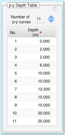
p-y Depth Table:

Note: This table is only if the ‘Auto-generate p-y Curves’ is not selected in this pane.

The ‘p-y Depth table’ is used to define the depth of the various p-y curves. The p-y curve for the selected depth is entered in the adjacent ‘p-y Table’ pane. 

Number of p-y curves

First select the ‘number of p-y curves’ using the up/down arrow.  This will add the appropriate number of rows in the table to populate

Up to 100 p-y curves can be specified.

Table:

You can double-click on the table cells to edit the content of the cells.

Only the ‘Depth’ column can be edited. 

Depth Column – This defines the depth of the p-y curve. p-y curves need to be specified at-least till the pile depth.

p-y Table:

Note: This table is editable only if the ‘Auto-generate p-y Curves’ is not selected in this pane.

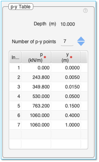
The ‘p-y Table’ defines the p-y curve points for the selected depth in the adjacent ‘p-y Depth Table’. 

Number of p-y Points

First select the ‘number of p-y points’ in the curve using the up/down arrow.  This will add the appropriate number of rows in the table to populate

Up 15 p-y points can be specified for each curve.

Table:

You can double-click on the table cells to edit the content of the cells.

The table consists of two editable columns –p and y. 

p Column – This defines the p values of the p-y curve.

y Column – This defines the y values of the p-y curve.

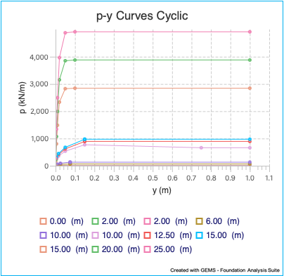
p-y Chart:

The p-y Chart plots the p-y curves based on the data in the adjacent ‘p-y Depth table’ and ‘p-y Table’. 

There are two options for plotting the curves.

a) Up to 20% of pile dia / up to pile dia.  Use the toggle switch to select one of the options.  If ‘Up to 20% of pile dia’ is selected, this option will plot the p-y curves with y values ranging from 0 to 20% of pile diameter.  This helps with better visualization of the p-y curves since most of the values lie within this range before the p-y chart levels off.

b) Selected depths / All depths.  Use the toggle switch to select one of the options.  If ‘Selected depths’ is selected, this option will plot only the p-y curve associated with the depth selected in the ‘p-y Depth Table’.  This option is useful to inspect a particular p-y chart.  By default, p-y charts for all the depths are shown in the graph. 

Soil Properties Tab > t-z Tab

Note: t-z curves are required only if ‘Axially Loaded Pile Analysis’ is selected in the Project Properties Tab.  Data in this tab is not used otherwise and can be skipped altogether if only ‘Pile Capacity’ or ‘Laterally Loaded Pile Analysis’ is required. 

The t-z curves can either be (a) auto-generated based on ‘soil properties’ and ‘pile dimensions’ or (b) user-defined. 

Auto-generate t-z Curves checkbox: Select this checkbox to autogenerate the t-z from the soil properties.  The values are autogenerated and populated in the ‘t-z Depth Table’ and ‘t-z Table’ on this pane when the ‘Compute’ option is selected from the menu-bar. The graph on this tab is updated. The auto-generated values are further used in the axially loaded pile analysis.

To specify user defined t-z curves, leave the checkbox unchecked. 

Compute t-z Curves button:  Click this button to autogenerate the t-z curves for the project. The data in the soil properties pane and pile dimensions pane is used for generating the t-z curves. 

Note: The existing values in the ‘t-z Depth Table’ and ‘t-z Table’ will be overwritten by the newly generated values. 

t-z Depth Table:

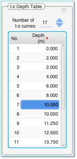
Note: This table is editable only if the ‘Auto-generate t-z Curves’ is not selected in this pane.

The ‘t-z Depth table’ is used to define the depth of the various t-z curves. The t-z curve for the selected depth is entered in the adjacent ‘t-z Table’ pane. 

Number of t-z Curves

First select the ‘number of t-z curves’ using the up/down arrow.  This will add the appropriate number of rows in the table to populate

Up 100 t-z curves can be specified.

Table:

You can double-click on the table cells to edit the content of the cells.

Only the ‘Depth’ column can be edited. 

Depth Column – This defines the depth of the t-z curve. t-z curves need to be specified at-least till the pile depth.

t-z Table:

Note: This table is editable only if the ‘Auto-generate t-z Curves’ is not selected in this pane.

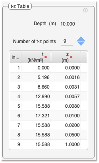
The ‘t-z Table’ defines the t-z Curve for the selected depth in the adjacent ‘t-z Depth Table’. 

Number of t-z Points

First select the ‘number of t-z points’ in the curve using the up/down arrow.  This will add the appropriate number of rows in the table to populate

Up 15 t-z points can be specified for each curve.

Table:

You can double-click on the table cells to edit the content of the cells.

The table consists of two editable columns – t and z. 

t Column – This defines the t values of the t-z curve.

z Column – This defines the z values of the t-z curve.

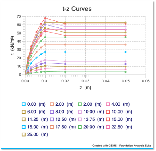
t-z Chart:

The t-z Chart plots the t-z curves based on the data in the adjacent tables.  

There are two options for plotting the curves.

a) Up to 20% of pile dia / up to pile dia.  Use the toggle switch to select one of the options.  If ‘Up to 20% of pile dia’ is selected, this option will plot the t-z curves with z values ranging from 0 to 20% of pile diameter.  This helps with better visualization of the t-z curves since most of the values lie within this range before the t-z chart levels off.

b) Selected depths / All depths.  Use the toggle switch to select one of the options.  If ‘Selected depths’ is selected, this option will plot only the t-z curve associated with the depth selected in the ‘t-z Depth Table’.  This option is useful to inspect a particular t-z chart.  By default, t-z charts for all the depths are shown in the graph. 

Soil Properties Tab > Q-z Tab

Note: Q-z curves are required only if ‘Axially Loaded Pile Analysis’ is selected in the Project Properties Tab.  Data in this tab is not used otherwise and can be skipped altogether if only ‘Pile Capacity’ or ‘Laterally Loaded Pile Analysis’ is required. 

The Q-z curves can either be (a) auto-generated from data in the ‘soil properties’ and ‘pile dimensions’ tab or (b) user-defined. 

If Q-z curve is ‘user-defined’, it needs to be specified at the depth corresponding to pile base. 

Auto-generate Q-z Curve checkbox: Select this checkbox to autogenerate the Q-z curve from the soil properties.  The values are autogenerated and populated in the ‘Q-z Table’ on this pane when the ‘Compute’ option is selected from the menu-bar.  The auto-generated values are further used in the axially loaded pile analysis.

To specify user defined Q-z curves, leave the checkbox unchecked. 

Compute Q-z Curves button:  Click this button to autogenerate the Q-z curves for the project. The data in the soil properties pane and pile dimensions pane is used for generating the Q-z curves.  Caution: The existing values in the ‘Q-z Depth Table’ and ‘Q-z Table’ will be overwritten by the newly generated values. 

Q-z Table:

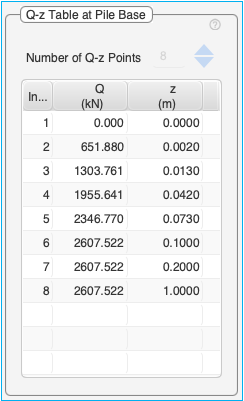
Note: This table is editable only if the ‘Auto-generate Q-z Curves’ is not selected in this pane.

The ‘Q-z Table’ defines the Q-z Curve for the depth corresponding to the base of the pile. 

Number of Q-z Points

First select the ‘number of Q-z points’ in the curve using the up/down arrow.  This will add the appropriate number of rows in the table to populate

Up 15 Q-z points can be specified for the curve.

Table:

You can double-click on the table cells to edit the content of the cells.

The table consists of two editable columns – Q and z.

Q Column – This defines the Q values of the Q-z curve.

z Column – This defines the z values of the Q-z curve.

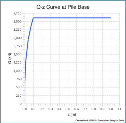
Q-z Curve:

The Q-z Curve plots the Q-z curves based on the data in the ‘Q-z table’. 

Option:

a) Up to 20% of pile dia / up to pile dia.  Use the toggle switch to select one of the options.  If ‘Up to 20% of pile dia’ is selected, this option will plot the Q-z curves with z values ranging from 0 to 20% of pile diameter.  This helps with better visualization of the Q-z curves since most of the values lie within this range before the Q-z chart levels off.

Load Cases Tab

The ‘Load Cases’ tab is used to enter details of the loading on the pile.

It is important to first specify the ‘Number of load-cases’ in the ‘Project Properties Pane’.  This will setup the appropriate number of tabs under the ‘Load Cases Tab’ for specifying the details of each load case. 

Each load-case should be entered in a separate tab (on the right-hand side).  Each load case tab consists of details of the load applied on the pile along with a loading diagram that graphically represents the same.

Load Case Description

Enter the description of the load case for your reference.  This is an editable text field. 

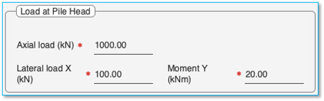
Load at Pile Head

Axial load

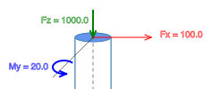
Specify the axial load applied on the pile at the pile head.  Compressive loads (+ve) values act downward while tensile loads (-ve) values act upwards. 

Lateral load

Specify the lateral load applied on the pile head. The load acts along the X direction. 

Moment

Specify the moment load applied at the pile head. The moment acts around the Y direction. 

Note: that counterclockwise moment is +ve.  If clockwise moment is to be applied, then prefix a –ve sign to the value. 

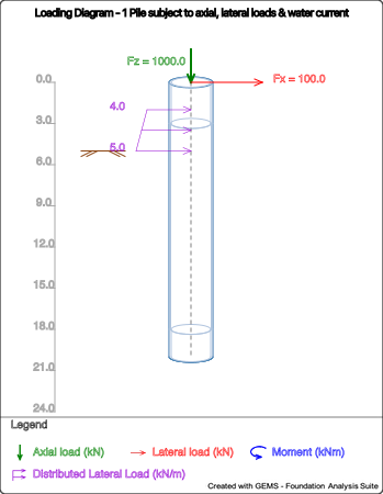
The figure above shows an axial load of 1000kN, lateral load of 100kN and a lateral moment of 20kNm applied at the pile head.

Include ‘self-weight’ in analysis

Select this checkbox if the weight of the pile is to be included in the analysis.  The weight of the pile is used in axial analysis only.  It is not taken into consideration for lateral analysis 

The “self-weight” of the pile consists of pile weight and plug weight and is taken from the ‘Self weight inputs’ pane in the ‘Pile Properties’ tab. 

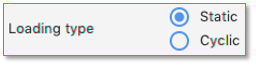
Loading type

Loading type can either be static loading or cyclic loading.  Use the radio button to select the option.  Cyclic loading is used to simulate long term effects of wave action on a long pile.

Additional Loads

Along with the load applied at the pile head, concentrated loads (axial load, lateral load, lateral moment) can be applied along the length of the pile.  In addition, a distributed lateral load can also be applied.   These can be useful for modelling wave action, water currents, loads applied on single buoy mooring piles. 

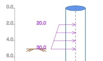
Distributed Lateral Load

The distributed lateral load can be used to model distributed loads along the length of the pile.  The loads can be triangular, uniform, or trapezoidal.  This is especially useful for modelling the effects of wave actions and water currents on the pile.

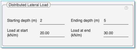
The distributed lateral load acts along the X direction. 

Specify the starting depth, ending depth along with the load at the starting depth and load at the ending depth.  If any of the values are left blank, then it is assumed that no distributed load is being applied. 

The figure above shows a trapezoidal load of 20kNm to 30kNm applied from a depth of 2m to 5m on the pile. 

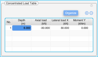
Concentrated Load Table

This table is used to specify the additional concentrated loads and moments applied on the pile along its length. 

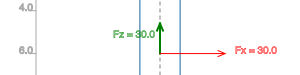
The example above shows a pile with 30kN tensile and 30kNm lateral load applied at 6m depth. 

Use the (+) and (-) buttons at the top of the table to add / delete rows to the Concentrated Load Table'. 

[Organize] button can be used to sort the values in ascending order of ‘depth’ and to clean up empty entries in the table. 

Table Columns:

Depth: Specify the depth where the load is applied.

Note: A total of 20 unique depths with axial loads can be specified for axial analysis across load cases.

Axial load: Specify the axial load applied at the point.  Compressive loads (+ve) values act downward while tensile loads (-ve) values act upwards. 

Note: Only the axial load applied at the pile head is included in the calculation of beam-column effect for lateral load analysis. 

Lateral load: Specify the lateral load applied at the point.  The load acts along the X direction. 

Moment: Specify the moment applied at the point.  The moment acts around the Y direction. 

Note: that counterclockwise moment is +ve.  If clockwise moment is to be applied, then prefix a –ve sign to the value. 

Right click on the table to bring-up the context menu to insert / delete rows in the middle of the table, cut, copy, delete and paste contents into the table.  It is also possible to copy the table from excel and paste the contents into this table.  Ensure adequate number of empty rows are added to the table prior to pasting contents from an excel table.

Loading Diagram

The loading diagram represents the axial load, lateral load, and a distributed lateral load (trapezoidal) applied on the pile for a load case.

Bibliography

Focht Jr., John A. Koch, Kenneth. J. “Rational Analysis of the Lateral Performance of Offshore Pile Groups.” Offshore Technology Conference. 1973. Paper N0 1896.

H. G. Poulos, H.G. and Davis E. H. Pile Foundation Analysis and Design. 1980, n.d.

Reese, et al. “Analysis of a Pile Group under Lateral Loading, Laterally Loaded Deep Foundations: Analysis and Performance.” ASTM, STP 835, 1984: 56-71.

Fleming. Piling Engineering. 2009.

“API RP2A.” WSD, 2000.

“Geotechnical and Foundation Design Considerations.” ANSI/API RP2GEO, April 2011, Addendum 1, 2014.

Reese, L.C., and W.R. Cox. “Field Testing and Analysis of Laterally Loaded Piles in Stiff Clay.” 5th Annual Offshore Technology Conference. Houston, Texas, April 1975.

Reese, L.C. “Analysis of Laterally Loaded Piles in Weak Rock.” Geotechnical and Geoenvironmental Engineering, 1997.

Turner, J. Rock-Socketed Shafts for Highway Structure Foundations. In:Program, N.C.H.R(Ed). A Synthesis of Highway Practice, Transportation Research Board of the National Academies, 2006.

Franke, Kevin W, and Rollins M Kyle. “Simplified hybrid p-y spring model for liquified soils.” Geotechnical and Geo-environmental Eng., no. 139(4) (2013): 564-576.

Matlock, H. “Correlations for design of laterally-loaded piles in soft clay.” 2nd Annual Offshore Technology Conference. Richardson, Texas, 1970. 577-594.

Rollins, K. M., T. M. Gerber, J. D. Lane, and S. Ashford. “Lateral resistance of a full-scale pile group in liquefied sand.” Geotech. Geoenviron. Engg, no. 131(1) (2005): 115-125.

Rollins, K. M., L. J. Hales, J. D. Lane, and W. M. Camp. “p-y curves for large diameter shafts in liquefied sand for blast liquefaction tests.” Seismic performance and simulation of pile. 2005b.

Peck, R. B., W. E. Hanson, and T. H. Thornburn. Foundation Engineering. New York: Wiley, 1974.

Seed, R. B., and L. F. Harder. “SPT based analysis of cyclic pore pressure generation and undrained residual strength.” H. Bolton Seed Memorial Symp. Richmond, BC, Canada: Bitech, 1990. 351-376.